BAM!

The concept of pseudoalignment was first introduced in Nicolas Bray’s PhD Thesis and is one of the core concepts behind the fast RNA-Seq quantification in kallisto.

A pseudoalignment of a read is simply a set of target sequences that the read is compatible with. Contrary to normal read alignment, where we specify where the read aligns and how, i.e. how the nucleotides in the read match up with the nucleotides in the target sequence. A more precise definition and discussion can be found in Lior Pachter’s blog post What is a read mapping.

The definition of pseudoalignment is crafted so that the output is a sufficient statistic for the basic RNA-Seq quantification model. As such, the focus is on sets of transcripts with counts rather than detailed alignments, and this makes pseudoalignments less intuitive than regular alignments, and harder to visualize.

Early on in the development of kallisto I started working on a way to report each pseudoalignment in a systematic way, namely to convert them to SAM records. This started only for debugging purposes, but we thought it was useful so we added it to the early releases. We called this approach pseudobam (even though the output was SAM, a text format which could be converted to BAM, a binary representation). In addition to reporting the set of targets the read aligns to we also included the position and orientation.

The issue was that SAM files are big and generating them took a long time, long by kallisto standards at least. Another annoyance was that they could only be computed using a single core, whereas regular kallisto can make use of multiple cores. Finally the output was only to transcriptome coordinates, since kallisto is by design annotation agnostic; it only requires transcript sequences and not the full genome or any knowledge of where those transcripts occur.

This has all changed now. In our latest release of kallisto (version 0.44.0) we output binary BAM files when kallisto is run with the pseudobam option. kallisto will make use of multiple cores when constructing the BAM file and additionally we report the posterior probability of each alignment in the BAM file. The posterior probability of an alignment is an estimate, based on the results of the EM algorithm that kallisto ran for quantification, of how likely the alignment was to have originated from that location¹.

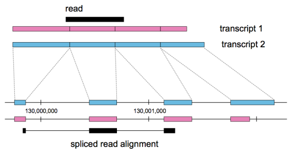
We also project the pseudoalignments down to a genome reference², producing a BAM file in genomic coordinates, where the pseudoalignments which were originally computed w.r.t. transcripts have been turned into spliced alignments to the genome.

The BAM files that kallisto produces are automatically sorted by genome coordinates and indexed, so that they can be viewed immediately in a genome browser such as IGV. This circumvents the need for Samtools to sort and index the BAM file prior to visualization, in particular, kallisto now provides a simple and efficient reads to visualization for  RNA-Seq analysis on windows machines.

When we were developing this we kept an eye on speed. Running kallisto and producing the BAM files took 24m11s using 8 cores on a file with 78M reads. When we tested this on unsorted reads generated by kallisto, using Samtools to sort and index required 13m45s using 8 threads. Although more thorough benchmarking is in order I think we can claim that we have the fastest reads-to-visualization pipeline currently available.

With your BAM files ready you can visualize your pseudoalignments, construct Sashimi plots and inspect the data interactively³.

IGV browser view of kallisto pseudoalignments of the LSP1 gene from RNA-Seq sample ERR1881406. The top panel shows a wiggle plot of coverage, with individual read pseudoalignments displayed below. Read pseudoalignments in the BAM file include the posterior probabilities in the ZW tag. The Sashimi plot shows the number of spliced reads identified by kallisto. The transcript structure is shown in the third panel.

When we’ve done differential expression studies using sleuth one of the things we do to verify the results is to plot the data for the top differentially expressed genes. We do this after having run a statistical test of every gene expressed. Similarly, we can now produce BAM files in genome coordinates to visulize the pseudoalignments and quality control them to ensure that our signal is not driven by artifacts or incomplete annotation.

Lior Pachter gave a keynote for the Genome Informatics where he showed some really exciting work on single cell RNA-Seq. Using this approach we could very quickly visualize the  pseudoalignment and see where in the CD45 gene the 10X reads were mapping. The visualization of the data allowed us to pick up on the fact that the annotation of 3′ UTR is probably incomplete for most genes, something you don’t “see” when staring at a sea of reads.

Notes

1. The concept of posterior probability of an alignment comes from eXpress and RSEM
2. This genome projection option was also available as a script in TopHat and RSEM.
3. The figures are from a poster I presented at Genome Informatics (full resolution poster)

Does NP-completeness have a role to play in Bioinformatics?

tl;dr: yes

Earlier this year I attempted to review a paper that had an NP-completeness result for aligning reads to de Bruijn Graphs. I say attempted, because I received an invitation to review the paper, was late, did a detailed review anyway and then found out that the editor had removed me as a reviewer when I tried to submit it. I sent the review anyway, but I don’t know if the authors received it.

This paper just came out a few days ago: Read mapping on de Bruijn graphs

Papers come and papers go, I didn’t think more of it until recently on twitter

The paper is bogus and the problem is certainly not NP-complete. See e.g. hybridSPAdes paper, it describes read-to-graph alignment

— SPAdes assembler (@spadesassembler) June 21, 2016

The language in this tweet is quite aggressive. Words like “bogus” and “certainly not NP-complete” do not (a) belong in a meaningful twitter conversation, (b) pinpoint any issue with the paper or (c) tell you why it’s wrong (after all the paper has a proof so it should be easy to tear that proof apart). I’m not going to go into point (a), that has been resolved on twitter.

What I want to get to are points (b) and (c). Before I do that, let’s look at the context. This paper has roughly two contributions, first the authors formulate a problem (I’ll get to what that means later) and show that this problem is NP-complete. Second the authors propose a quite reasonable heuristic that they show works well in practice and test on real data.

The formulation of the high level problem of aligning reads to a graph is as follows

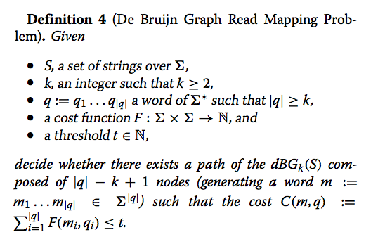
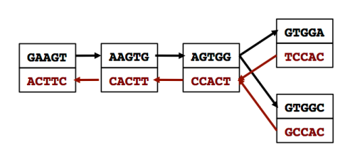
Basically what this means is that the question is given a read and a graph is there a path in the graph, whose sequence spells out something close () to the read . There is a similar formulation for the general case of a graph read mapping problem, where the nodes are not constrained to be -mers in a de Bruijn Graph.

This seems like a reasonable formulation of the problem we really want to solve and quite close to the type of alignment problems we know how to deal with when aligning to a single reference sequence.

At this point it’s worthwhile to consider a different problem which plays a role in genomics (assembly), namely the Hamiltonian path problem. It is a problem which turns out to be NP-complete, yet it’s close relative, the Eulerian cycle problem is easily solved. This distinction is of value in guiding modeling choices for assembly and in algorithm design.

In the case of read alignment to de Bruijn graphs, the authors prove that their problem formulation is NP-complete. I was skeptical so I set out to see if it had bugs, it didn’t.  Then I carefully checked whether it relied on having a large alphabet, nope the proof works with 4 letters. So after much huffing and puffing the proof held and I was convinced. In my review I simply noted

discussion of NP-completeness vs. heuristics: The structure of the DBG, and even
the contig graph is quite specific and not something we would expect to see in practice. The reduction to the Hamilton path also relies on having very long reads, whereas BGREAT is mostly focusing on short reads. Additionally there are several examples where random instances of problems are (provably) solvable using heuristics. I feel that there needs to be a better segue between the NPC result and jumping right into the description of BGREAT.

Any proof of NP-completeness involves showing that the problem you are dealing with now is harder than a problem previously shown to be in NP (and also you should be able to check proofs of it being in NP in polytime). When you do this you take an arbitrary instance of the other problem (in this case a TSP variant) and you encode it in a very special way as a new problem such that if you solve your new problem you can obtain a solution to the old one.

There are two points to make. First the new problem you see (in this case the de Bruijn Graph and the read ) can be quite weird and not something we expect to see in practice.

The second point I wanted to make is that NP-complete isn’t just about problems being hard, but that the problem is too expressive. This is something I remember Manuel Blum talking about when I first learned NP-completeness properly, I didn’t quite get it at the time, but now I tell myself I do. The issue of expressiveness is useful because it tells us if we are not careful we can accidentally make our problems too hard.

Anyway, that was quite the detour and we haven’t got to the real question posed in the title. Should we really care about NP-complete results in Bioinformatics, i.e. regardless of whether it is true or not (it is in this case), should we let it influence our work, the formulations we propose or new algorithms or whatever.

I’ll argue that the answer is yes, at least in this case. It’s too easy to dismiss this as something from theoryland that has no bearing on reality, just like we routinely solve incredibly large instances of TSP or find cheap flights online (you didn’t click the link above, did you?).

In this specific case the theory to reality disruption happens because 1. the encoding creates a de Bruijn Graph which is quite convoluted and nothing like what we observe in reality, 2. the read constructed in the encoding doesn’t occur in the graph, in particular it doesn’t have to share a single -mer with the de Bruijn Graph and 3. the distances can be quite big (close to  SHTseq levels) and the differences can be selected by an adversary. Even if you could find the best alignment, arguing that it’s biologically meaningful it going to be quite hard.

So we focus on the easier problems, like reads that actually came from the graph or something close to it with not too many errors. Hence the heuristics.

The takeaway is that if we try to solve the general problem, without any restrictions on distance or matching k-mers or anything we cannot guarantee a polynomial time solution unless P=NP.

This is not to say that NP-completeness will always be the right theoretical abstraction to work with. In genome assembly several problems have been proposed as “capturing the essence” of the problem, let’s pick Shortest Common Superstring as our straw man argument. The problem is NP-complete, but it ignores the coverage of repeats when it comes to assembly and so it doesn’t use all the information available. But we cold also ask a different question along the lines of “For this particular genome, how deep do I have to sequence and how long do the reads need to be so that I can solve it with tractable algorithms?”, this is sort of the information theoretic view of assembly, rather than the complexity theoretic view. This is the sort of view that David Tse’s group has been working on.

Thinking about this again I just realized that there is/could be a connection to a previous body of work on graph BWT methods. Notably, the seminal paper by Sirén et al. One of the issues with this approach is that it tends to blow up in memory, when faced with complex variant graphs like chr6 (which contains the infamous MHC region). The advantage of the extended xBWT method is that it doesn’t require to find exact matching k-mers, but the matches can be extended base-by-base just as in regular BWT matching (FM-index to be technically correct). I’ve thought about if there is a way around this issue and my MS student, Tom Schiller,  gave it a try, but I don’t think it’s easily solved. Perhaps it is inevitable since it get’s you closer to solving the general problem, which we know is NP-complete.

And this is the real value of NP-completeness for practitioners, it tells you that some problems are so expressive that trying to solve the general case is not going to work.

[Note: there are some issues with the BWT to NP-completeness connection, the extended xBWT requires the graph to be a DAG, I haven’t checked carefully whether the reduction works with a DAG or not. Also even if we had the extended xBWT data structure it’s not necessarily true that we can find an alignment with any cost function on poly-time. This is more like a hunch or an educated guess.]

 

Building Binaries for Bioinformatics

tl;dr there is a recipe for compiling binaries at the end

When it comes to working in bioinformatics, it is the best of times and it is the worst of times. For developers we have tons of modern tools, polished libraries, github and twitter and a sane extension of c++ called c++11. On the other hand we have clusters. Moreover, users have clusters that they don’t control, can’t install modern compilers (and by modern, I mean like two years old), can’t install libraries and compiling without root is pain.

I run a cluster which runs on the rocks cluster system. The newest version at the time was based on Centos6, the compiler was gcc 4.4, even old at the time. The reason is that distributions are reluctant to use the latest compilers and so users are stuck with old technologies.

How bad can it be? Well you lose out on c++11, to compile c++11 code you need gcc 4.8.1 or later for everything to work. Earlier versions of gcc can handle some of the features, but it’s not worth using them. I mean as the name implies c++11 was ready four years ago!

With c++11 I find myself much more productive as a programmer, with nice things built, good abstractions that get compiled to very fast code. I’m never going back. All of this comes with the cost of having to use a decent compiler. This means that you lose a lot of users because they can’t compile your code and the only way out is to release a binary version.

Binaries on Linux

Linux is wonderful, but it’s not the happy wonderland we would like to believe because distributions don’t always use the same versions of libraries, mostly libc, pthreads and friends. So when you create a binary to distribute you have to statically link against all your included libraries because you can’t rely on them being installed on the target system.

I ran into this problem when trying to create a binary for kallisto. The problem was that the HDF5 library had to be statically linked, but the pthreads library had to be dynamically linked. I spent a few nights trying to get it to work but nothing worked.

Holy Build Box

Then, on twitter, Heng Li tweeted about the Holy Build Box that promised a way to build binaries on linux that would work on any system. Long story short, it worked and here’s the recipe.

First the solution is built on top of docker, so you need a machine where you are root. I had an Ubuntu 14 desktop lying around so I installed the latest docker version and started reading the manual. If you are trying to build your own binaries I would recommend starting with the script below, modifying it as appropriate and reading through the manual.

Building kallisto

To build the binary we simply use a build script that takes care of everything, I only assume that I have the source files and the hdf5 library files in the current folder.

The first script is comp_kallisto.sh

docker run -t -i --rm \
  -v `pwd`:/io \
  -e CC='ccache gcc' \
  -e CXX='ccache g++' \
  -e CCACHE_DIR='/io/cache' \
  phusion/holy-build-box-64:latest \
  bash /io/build.sh $1

It takes as argument the version and passes it on to the build script build.sh. The -t -i --rm arguments show the output of the docker run and tear down the instance when we’re done, -v `pwd`:/io mounts the current directory as /io so we can transfer files in and out between the machine and the docker instance. The -e parameters set environment variables to cache the compilation, this is useful if you need to compile hdf5 over and over again until everything works. phusion/holy-build-box-64:latest is the name of the docker image, if you don’t have it docker will download it which should only take a few minutes.

What this image has is an old Centos 5 system with the latest compiler (well gcc 4.8.2 anyway) libstdc++ available only as static and fairly old libc and phtreads libraries. This means that if we link against those the binary will work on any newer system.

The build.sh script does all the work

#!/bin/bash
set -e

VER=$1
if [[ -z $VER ]]; then
  echo "specify version"
  exit;
fi

# Activate Holy Build Box environment.
source /hbb_exe/activate

set -x

# Install static hdf5
tar xfz /io/hdf5-1.8.*
cd hdf5-1.8.*
env CFLAGS="$STATICLIB_CFLAGS" CXXFLAGS="$STATICLIB_CXXFLAGS" \
  ./configure --prefix=/hbb_exe --disable-parallel \
  --without-szlib --without-pthread --disable-shared
make
make install
cd ..

# Extract and enter source
tar xzf /io/v${VER}.tar.gz
cd kallisto-${VER}

# compile and install kallisto
mkdir build
cd build
cmake ..
make
make install

# copy the binary back
cp /usr/local/bin/kallisto /io/kallisto_bin_${VER}

Since we’ve mounted the current directory as /io we simply extract the hdf5 code, build a static library with the correct parameters and install system wide. We don’t have to worry about cleaning up the mess because this “system” is going down in a minute. Plus inside docker we are root so we can do whatever we feel like. Once the hdf5 library is ready all the dependencies of kallisto are satisfied and we build it from the source and install the binary. Finally we copy the new binary back to the /io folder and exit the docker image. Once the script fininshes, the docker image goes down and with it all changes made. The end result is a binary that works on any linux system.

The Holy Build Box comes with some static libraries such as libz, but anything else you’ll have to build yourself. You can also run docker directly and get a shell just by running bash instead of bash build.sh and try it out there manually.

BamHash and some insights from information theory

We have a new preprint out for a tool called BamHash. I’ll get to what it does and how it works in a bit, but first the why.

This tool was built because we needed it at deCODE and couldn’t find anything else that could do it. The basic problem is that we have DNA sequenced on an Illumina machine producing FASTQ files, which are then pushed into the pipeline, processed, cuddled, fed locally grown produce and after some bioinformatics magic we get a shiny BAM file.

FASTQ files storing raw reads are big and ugly, whereas BAM files are small, sorted, indexed and just better. For a 30x coverage Human genome the BAM file will be about 70G, the raw FASTQ file is even worse. Multiply that by the number of individuals sequenced and you get, uh, a lot.

Obviously we want to get rid of the FASTQ file, and it is perfectly safe to do that because the BAM contains all the information in the FASTQ file. Worst case scenario: we could always recreate the FASTQ file from the BAM file if needed.

To illustrate the question consider the following conversation

paranoid me: is it safe to delete that FASTQ file?
me: what?!?, I just explained why it was safe why are you asking again?
paranoid me: well, something could have happened in your pipeline
me: is there something wrong with my pipeline?
paranoid me: or the disk system
me: I haven’t heard of anything, do you know something I don’t?
paranoid me: maybe there were hiccups and you dropped a few reads
me: no, you don’t understand, we have a pipeline
paranoid me: can you really be sure that all the reads in the FASTQ file made it to the BAM file?
me: now you are just being paranoid
paranoid me: “Yes I’m paranoid – but am I paranoid enough?” [source]

So how can we know if the reads in the FASTQ file are exactly the same as the reads in the BAM file? A simple solution is to just compare the two sets, but that would take too much time, plus we would have to keep everything in memory or write to disk and it’s really an overkill.

A simpler way is to construct fingerprints for the FASTQ and BAM files based only on the set of reads. The exact same reads appear in both files, but in different order. So the basic idea is to compute a hash value for each read and reduce the set of hash values to a single fingerprint. Reduce here means to apply some reduction operation such as a sum or XOR. As long as the binary operation is commutative the final result is independent of the order. Thus we settled on something simple, MD5 has of each read and add up all the values mod 2^64. Change one byte in your reads and you’ll get a different value.

The program is very efficient, on par with reading a BAM file with samtools and counting the lines. Now just stick this at the front and end of your pipeline and check that the input FASTQ and output BAM have the same fingerprint. If they match, delete that sucker. If they don’t, you have issues.

But wait there’s more

I was describing this result to Harold Pimentel who asked a natural follow-up question “since we like to throw away reads, is it possible to find if the FASTQ reads are a subset of the BAM reads”. The easy answer is yes, just do the naive thing and compare the sets directly. So the hard question is, can we find a fingerprinting method that will solve this problem.

I had no idea whether this was possible until I reframed the question. Instead of thinking about this as a computational problem let’s think about this as a communication problem from information theory.

Alice and Bob start doing bioinformatics

In this setting we have Alice holding a FASTQ file with reads, and BOB has a BAM file with reads, . They want to find out if using minimal communication. This is equivalent to finding out if . Any fingerprint method can be turned into a protocol where Alice sends the fingerprint and Bob compares the fingerprints and answers yes or now. The general setting where Alice and Bob can talk interactively allows for more complicated methods. [edit: the direction was wrong, BAM are supposed to be subsets of FASTQ in a practical setting, for the lower bound you just reverse the roles of Alice and Bob, they won’t mind]

The good news is (if you are a theorist, otherwise this is bad news) that this is simply the set disjointness problem and it turns out that the lower bound for the amount of communication that is needed is , even if we allow randomness and some small probability of failure.

In other words, no, there is no way any general fingerprinting method can find out if the BAM reads are a subset of the FASTQ reads. The fingerprint would have to be the size of the input which defeats the purpose. I added the word general, since there might be something clever you can do if you were told that only a handful of reads are missing or if you knew something more about the input, but let’s not go there.

BamHash ~ EQ

If we go back to BamHash, the fingerprinting method is answering the question whether , which it called the EQ problem. The EQ problem has a lower bound of for deterministic communication, i.e. no randomness and zero probability of failure. However the EQ problem has a bit solution when we allow randomness, and this is pretty much what BamHash is doing.

Dear assemblers, we need to talk … together

This post was co-authored by Michael R. Crusoe @biocrusoe and thanks to Shaun Jackman @sjackman for discussions and reading the draft.

tl;dr we need a common file format for contig graphs and other stuff too

The state of assembly software right now is essentially dominated by a few end-to-end solutions. These include SPAdes, ALLPATHS, ABySS, and SOAPdenovo (if your tool is not here, don’t take it the wrong way). This integration is good for consumers who want good methods that get them from raw fastq files to an assembled genome.

On the other hand this tight integration is not a good situation if you want to get into the assembly business. Here there are two scenarios which make entry into the field difficult. First if you have some good ideas about how to improve some part of the assembly process, you have two choices: a) write an assembler from scratch, b) try to modify the some of the programs mentioned before or work your way around them. The second scenario arises when you have a solution along the lines of “oh, I’ll just do an assembly with some minor modifications and the tweak the output a bit”.

The solution to these problems is to break up the “assembly” problem to a few well defined pieces. The analogy we should be thinking about is what is done in variant calling. In this case the process goes from raw reads to aligned reads in BAM files, then every variant caller reads the BAM file and spits out a VCF (say what you will about VCF, but at least it is a file format). This is exactly what the field of assembly needs right now. A few file formats that capture the common tasks that every assembler goes through.

The common tasks are

1. Create a graph (de Bruijn/overlap/contig/string … )
2. Simplify the graph
3. Map reads to graphs
4. Produce an assembly

Some of the assemblers do these steps with several programs, SOAPdenovo and ABySS for instance have a separate program for each part. Modularity at the software level is great, but it doesn’t allow practitioners to mix and match across different software platforms.

The best way to open up the field is to embrace the Unix mantra that everything is a file. A corollary of this is that the best API is the file. And this is the key point here. How you do 1,2,3, and 4 shouldn’t matter and shouldn’t be standardized, but rather the intermediate files between 1 and 2, etc. Right now we have good file formats for before point 1, namely FASTQ files, and after 4, either FASTA or FASTG.

What is missing is a file format and an agreement across the field to use those for the intermediate results. Many of the programs have these intermediate files, but they are often tied to a particular representation.

We need a common file format for the contig graph and read alignment to a contig graph. The graph format would take care of 1-2 and 2-3, since the output is a graph in both cases. Similarly the mapping of reads would allow you to go from 3 to 4. Once we have common file formats we would be free to choose whatever program for performing any of these steps.

Perhaps you would want to write a new algorithm for resolving repeats using next-next-next-generation sequencing you could take as input a contig graph from the old days and combine that with your new 74.5% error rate long-long read stuff. End users could then use your method with any assembler they think is doing best at the moment.

Let’s take a more concrete example and say you want to build an RNA-seq assembler, first step is to take reads and generate contigs. All you would have to do is pick a contig assembler and tell it to not worry about aggressive error correction, assumptions about uniform coverage and all sorts of fancy stuff and just give you the graph, you can take it over from there.

This brings me to the next issue which is graph read alignment. This entails taking reads and mapping them against the graph. Instead of mapping to a linear sequence like a chromosome in a well defined assembly, or just a contig/scaffold, we are looking for an alignment to a path in the graph. Of course paths in the graph should correspond to a contiguous stretch of the underlying genome or transcriptome. The alignment will necessarily be fragmented when you have reads that can span multiple contigs.

A tool that can take as input a graph and raw reads and map the reads to the graph would be very valuable. This is currently something people are working on, both within and outside assemblers, but what is missing is the interoperability in terms of (again) the graph file format and more importantly the alignment format.

So what is the solution? I have no idea.

Ok, that’s not right, I have a few ideas, but I’m willing to change my mind.

First things first, the graph file format. There is already a graph file format for sequences, FASTG. But I have a few issues. It was meant as a format for representing variability in the final output of an assembly, e.g. SNPs, indels, tandem repeats etc, that doesn’t really break up a contig. Both SPAdes and ALLPATHS output FASTG files, but from what I can tell they don’t use it for intermediate results. Also there is no notion of coverage in FASTG, but you can put that as a property of the edge. Also, the graph stores sequences on the edges instead of nodes. I don’t like it, but if you can convince me I’m wrong I’ll reverse my position.

But unfortunately there is very little library support for FASTG. Writing a full parser for it is not impossible, but if you look at the standard you’ll see that there’s plenty of work to do. One idea would be to restrict the contig graph to a smaller subset of the FASTG standard. Essentially this would mean no funny business in the sequence (read the standard and you’ll be amazed at what is possible), so that is still a valid FASTA file (sort of), and encode the coverage and other information in the comment. So a simple example would be

>A:B:cov=10;
GATTA
>B:C':cov=9;
AC
>C::cov=19;
T

Another way to represent the graph is the way ABySS does it. Hat tip to Shaun Jackman for telling me about this (but he works on ABySS and is a part of the establishment, so take this with a grain of salt). The idea is to keep contigs in a FASTA file and have a separate graph file in the Graphviz dot file format, you can see the nitty gritty details. The key here is to use a subset of the dot file format popularized by Graphviz. This buys you a whole lot of library wonderfulness and plenty of programs that read the format. Essentially you keep track of edges of the graph by listing them in a bidirectional format so “A+” ->  “B+” is forward strand of A is followed by forward strand of B, whereas “B+” -> “C-” is forward strand of B is followed by reverse complement of C. If you don’t know why the bidirectional stuff is needed you have to read Gene Myers’ String Graph paper. We’ll wait.

What is really cute is that you can specify properties of the edges like overlap, which allow you to store more context in sequences for the contigs. If the above example had been formed with a de Bruijn graph with k=4, the resulting contigs might have been

>A
GATTA
>B
TTAC
>C
TGTA

and the dot file would be

digraph g {
A+ -> B+ [overlap=3]
B+ -> C- [overlap=3]
}

The advantage of this way is that both dot files and fasta files are standard with libraries that can parse this information. Also since the sequence and the graph are separated it allows you to work with the graph directly without loading the sequence. For instance if you would want to trim down the graph or only work with a particular subgraph you would only need to load the graph file, do your graph theory business and then work with the small subgraph. If you need to load a subset of the sequences you can have your FASTA files indexed and load only the sequences that you need.

I’ll leave the issue of graph alignment and how to represent the output until later. For now I just wanted to throw it out there because I think this is something that needs to happen. The implementation for outputting the graph files is not a lot of work if you have an assembly program, what’s keeping them back is that there haven’t been any requests for doing it and no common file format.

Let’s talk about this, either in comments, blog posts or on twitter. I really don’t care which format we use, as long as we can have a common one.

 

Additional thoughts:

This has been preached by the small tools manifesto for a wider class of problems.
Earlier this year there was discussion about similar issues in the context of scaffolders.

 

late update (july 22): Heng Li has a new proposal on his blog on a file format, the discussion in the comments is quite active.

Analyzing data while downloading

I’m at HiTSeq14 and ISMB14 and just gave my KmerStream talk yesterday. The best thing about giving a talk is that people look at what you’ve been doing in new ways. So yesterday I was talking to Shaun Jackman about potential applications and I joked that you could analyze data while downloading it.

And then I thought about it for a bit, implemented it into KmerStream. It’s now on the github repository under the online branch. It just adds an –online flag which will print an estimate of the k-mer statistics every 100K reads.

What you can do is then download data sets, tee the input and process it at the sama time. It is a bit of a hack, with the shell command, but just looking at it run is worth it.

curl -s  http://gage.cbcb.umd.edu/data/Staphylococcus_aureus/Data.original/frag_1.fastq.gz | tee frag_1.fastq.gz |  gzcat -f | ./KmerStream -k 31 -o tmp --online /dev/fd/0

So what is happening is that curl -s downloads the data and doesn’t print any progress reports and prints to stdout. tee will take the stdout and save to the file, gzcat takes the input and unzippes it (use gzcat on mac and regular zcat on linux). KmerStream doesn’t read from stdin, but you can always read from stdin through the special file /dev/fd/0 so that fixes it.

Here is the output in all its glory, but it doesn’t do it justice compared to seeing it in action.

100K reads  -- 1009K repeated, 4M distinct, 3M singletons, 6M total k-mers processed
200K reads  -- 1M repeated, 7M distinct, 6M singletons, 13M total k-mers processed
300K reads  -- 2M repeated, 11M distinct, 8M singletons, 20M total k-mers processed
400K reads  -- 2M repeated, 13M distinct, 10M singletons, 26M total k-mers processed
500K reads  -- 2M repeated, 15M distinct, 12M singletons, 33M total k-mers processed
...

It is also possible to break off once you’ve seen enough and keep what you’ve downloaded. If it is  a gzipped file, it is a bit broken since the end is missing. However the data is still there and you would need to fix the fastq file by removing the broken read.

deBuGging de Bruijn Graphs

In the previous posts I showed a toy implementation of a dBG assembler and then found that something was wrong with the edge cases. I’ll show how to fix these edge cases by testing this on circular contigs and something similar.

It turns out to be much easier to work with short reads and small values of k. In this case I’ll be working with k=5. Our test case will be one read for the entire contig

TTCAGCGATAACATCTTTCA

When we feed this to the assembler we get (I put cyclic.fq twice since by default I’m filtering k-mers with a coverage of 1)

$ python dbg.py 5 cyclic.fq cyclic.fq
>contig0
TCTTTCAGCGATAACATCTTTCAGCGATAACATCT

What?!? Ok, this is not what we wanted. The good news is that our contig seems to be inside the result.

TCTTTCAGCGATAACATCTTTCAGCGATAACATCT
   ||||||||||||||||||||
   TTCAGCGATAACATCTTTCA
                   ||||||||||||||||
                   TTCAGCGATAACATCTTTCA
|||||||
TCTTTCA

Only it’s there twice wrapped around the result. There are two places where this could have gone wrong
a) in the function get_contig_forward(d,km), b) in the function get_contig(d,km). We should first check that get_contig_forward is doing the right thing. We can run the python script and get an interactive shell afterwards by doing

$ python -i dbg.py 5 cyclic.fq cyclic.fq
>contig0
TCTTTCAGCGATAACATCTTTCAGCGATAACATCT

>>>

The -i keeps the python session open with all the variables and functions in place. We can check the function by doing

>>> get_contig_forward(d,'TTCAG')
['TTCAG', 'TCAGC', 'CAGCG', 'AGCGA', 'GCGAT', 'CGATA', 'GATAA', 'ATAAC', 'TAACA', 'AACAT', 'ACATC', 'CATCT', 'ATCTT', 'TCTTT', 'CTTTC', 'TTTCA']

Which are the k-mers in "TTCAGCGATAACATCTTTCA", ok, so nothing odd here.

Now get_contig(d,km) has two function calls to get_contig_forward. We assume that km is in the middle of some contig, so we get the forward extension with

c_fw = get_contig_forward(d,km)

which should be the part of the contig from km to the end. We get the backward extension with

c_bw = get_contig_forward(d,twin(km))

we reuse the forward function and call it with twin(km) so that we get the reverse complement of the first part of the contig. Now we see why this fails since,

>>> get_contig_forward(d,twin('TTCAG'))
['CTGAA', 'TGAAA', 'GAAAG', 'AAAGA', 'AAGAT', 'AGATG', 'GATGT', 'ATGTT', 'TGTTA', 'GTTAT', 'TTATC', 'TATCG', 'ATCGC', 'TCGCT', 'CGCTG', 'GCTGA']

which is the contig for "CTGAAAGATGTTATCGCTGA", the reverse complement of the contig we started with. So we need to fix this by checking if this is a circular contig.

But before we fix this we should fix a nastier error.

Our test case is a tiny contig "ACGTTGCA" and when we run our program the output is "TTGCAACGTTGCAACGTTG"

Which is really wrong. Checking get_contig_forward as before the output is

>>> get_contig_forward(d,'TTGCA')
['TTGCA', 'TGCAA', 'GCAAC', 'CAACG', 'AACGT', 'ACGTT', 'CGTTG', 'GTTGC']

which corresponds to the contig "TGCAATGCAACGT". But the result should only have been 4 k-mers, but we got 8? In fact the dictionary for all k-mers has only 8 k-mers and that’s counting both forward and reverse. If you look at the original contig "ACGTTGCA", you’ll see that 'TTGCA' is the last k-mer and the next k-mer in the output is 'TGCAA' which is the reverse complement. If you’ll remember from the last post the 6-mer 'TTGCAA' is its own reverse complement, so what we have here is really a hairpin. But it’s not just a hairpin because the first k-mer 'ACGTT' has 'AACGT' as a neighbor so there are two hairpins at both ends of the k-mer.

My head hurts, lets draw this

ok, so now we see what just happened. We started in the top from left to right and went backwards in the reverse complement and round again. The check for loops in get_contig_forward was to see if the next k-mer to add was already in the contig, we should have checked for the twin as well.

Now if we redraw the figure by dropping the twins of each k-mer, but keeping the edges shown in red we get.

So this is not a circular contig in the regular sense, but sort of “first you go one round on one side and then another on the other side, only to come back at the beginning”. Hah! I know lets call it a Möbius contig.

Fixing things.

We update the get_contig_forward definition from

def get_contig_forward(d,km):
    c_fw = [km]
    
    while True:
        if sum(x in d for x in fw(c_fw[-1])) != 1:
            break
        
        cand = [x for x in fw(c_fw[-1]) if x in d][0]
        if cand in c_fw:
            break
        
        if sum(x in d for x in bw(cand)) != 1:
            break

        c_fw.append(cand)

    return c_fw

to

def get_contig_forward(d,km):
    c_fw = [km]
    
    while True:
        if sum(x in d for x in fw(c_fw[-1])) != 1:
            break
        
        cand = [x for x in fw(c_fw[-1]) if x in d][0]
        if cand == km or cand == twin(km):
            break # break out of cycles or mobius contigs
        if cand == twin(c_fw[-1]):
            break # break out of hairpins
        
        if sum(x in d for x in bw(cand)) != 1:
            break

        c_fw.append(cand)

    return c_fw

plus it is a bit less inefficient since we only compare cand to the last or first k-mer to the candidate extension.

We also fix get_contig by checking if the last k-mer in the forwards extension is a neighbor of the first one.

From

def get_contig(d,km):
    c_fw = get_contig_forward(d,km)
    c_bw = get_contig_forward(d,twin(km))

    c = [twin(x) for x in c_bw[-1:0:-1]] + c_fw
    s = c[0] + ''.join(x[-1] for x in c[1:])
    return s,c

To the slightly more readable

def contig_to_string(c):
    return c[0] + ''.join(x[-1] for x in c[1:])

def get_contig(d,km):
    c_fw = get_contig_forward(d,km)
    
    c_bw = get_contig_forward(d,twin(km))

    if km in fw(c_fw[-1]):
        c = c_fw
    else:
        c = [twin(x) for x in c_bw[-1:0:-1]] + c_fw
    return contig_to_string(c),c

The source code has been updated on github as well as the test cases above. Now for next time we’ll, uh, I have no idea, just tell my on twitter: @pmelsted

Edge cases in de Bruijn graphs

In the previous post I showed a simple implementation of a de Bruijn graph assembler. This implementation is mostly correct, for some definition of mostly.

One of the key differences between the original combinatorial definition of a de Bruijn graph and what we use for assembly is that a) the de Bruijn graph contains every k-mer and what we use for assembly is just a subgraph of the big one (this is just a technicality) but more importantly b) we make no distinction between a k-mer and its reverse complement, frequently referred to as its twin in assembly-lingo.

This gluing of a k-mer and its twin means that we can do one of two things. Either we can keep both copies and store the directed graph.

This is much easier to work with and think about since we can see that the edges go in opposite directions. So if we have an x->y edge then we must have a twin(y)->twin(y) edge as well (shown in red). As a convenient notation I’ll refer to the reverse complement of x by ~x from now on. Also if k is an odd number then every k-mer is distinct from its twin (to see why just think about the middle character).

The downside is the memory usage is doubled. Since memory is a huge issue in assembly we generally want to keep only track of one of the two k-mers. This is done by appointing one of them to be the representative k-mer, usually the lexicographically smaller of the two (a fancy way of saying whichever comes first in alphabetical order), but as long as it’s consistent it doesn’t matter how it’s done.

Although you don’t wan’t to represent it this way in code it is much easier to think about both copies of the k-mers, like above, rather than only the representative.

Edge cases

So when does the previous code not quite work. It has to do with the our non-existent, and therefore not rigorous, definition of a contig. A contig is a maximal linear path in the de Bruijn graph. One nice observation is that every k-mer, x, is contained in exactly one contig, and the same goes for the twin of x and it should be in the same contig. Note that a contig might just have one k-mer in it. The linear condition says that each internal vertex on the path has out-degree 1 and in-degree 1. To put this another way, x->y is in a contig if there are no other x->b or a->y edges.

This condition covers most cases, namely the ones where x,y,~x,~y are all distinct. Since k is odd we’re guaranteed that x and ~x are distinct. So what happens if x and y are the same, can that really happen? This would imply that the last k-1 bases of x are equal to first k-1 bases of x. The only way this can happen is if we have x="AAA...A" or any other repetition.

The other case is if x and ~y are the same so x-> ~x. In this case the last k-1 bases of x are equal to the first k-1 bases of ~x. So the first base of x doesn’t matter, since it’s the complement of the last base of ~x.

However we have that x[1:] = (~x)[:k-1] = ~(x[1:]), I’m using python string slice notation where x[1:] is from position 1 (we start at 0) onwards and x[:k-1] is the first k-1 bases. This shows that the (k-1)-mer x[1:] is its own twin, which was exactly the possibility we wanted to avoid by choosing k to be odd. This also means that the (k+1)-mer of x+y[k] which represents the edge x->y is a self-twin as well. As an example we can have x="CAATT" so then ~x="AATTG" and then we can see that x->~x.

For even k we can characterize the k-mers that are self-twins by specifying the first k/2 bases and the remaining k/2 will be the reverse complement of the first k/2, this means that there are such k-mers. So the number of k-mers is , and for k odd we have distinct representatives, but for k even we have distinct representatives. [edit 4/30/15, thanks to Lior Pachter for noticing an arithmetic bug]

But wait, there’s more

When we said that we made no distinction between x and ~x and treat them equally we have to be careful when defining edges and degrees and actually start using bidirected edges, but that I’ll leave that as an exercise for the reader or a later post.

Next time we’ll see how to fix the code to handle these edge cases properly. There is an additional bug in the code, although you could say it’s a feature, it has to do with circular contigs and hats off to you if you can find it. [read the follow up]

Naive python implementation of a de Bruijn Graph

De Bruijn graphs are widely used in assembly algorithms and I guess writing your own assembler is a rite of passage. Hoping to get some answers I got this question from Mick Watson. Since I had a script lying around that I used for validation I thought I would share it.

For contig/string graphs, what is the advantage of having the sequence in edges (like FASTG) rather than the vertices (de Bruijn style) ?

— Pall Melsted (@pmelsted) November 23, 2013

So let’s see how this is done. First we’ll need to work with k-mers, which are substrings of a fixed length k. Since we’re keeping this as simple as possible we’ll use python strings for k-mers. Some functions to work with those

import collections, sys
from Bio import Seq, SeqIO, SeqRecord

def twin(km):
    return Seq.reverse_complement(km)

def kmers(seq,k):
    for i in xrange(len(seq)-k+1):
        yield seq[i:i+k]

def fw(km):
    for x in 'ACGT':
        yield km[1:]+x

def bw(km):
    for x in 'ACGT':
        yield x + km[:-1]

The yield statement in python gives us an iterator object, so we can write stuff like

for x in fw("ATAT"):
    print x

which will print TATA, TATC, TATG and TATT, i.e. all forward neighbors of the k-mer “ATAT”. If we need to convert the iterator to a list the easiest thing to do is list(fw("ATAT")).

To keep track of all the k-mers we store them in a dictionary that keeps track of the coverage. For each k-mer we’ll add the reverse complement as well.

def build(fn,k=31,limit=1):
    d = collections.defaultdict(int)

    for f in fn:
        reads = SeqIO.parse(f,'fastq')
        for read in reads:
            seq_s = str(read.seq)
            seq_l = seq_s.split('N')
            for seq in seq_l:
                for km in kmers(seq,k):
                    d[km] +=1
                seq = twin(seq)
                for km in kmers(seq,k):
                    d[km] += 1

    d1 = [x for x in d if d[x] <= limit]
    for x in d1:
        del d[x]

    return d

Line 2 defines a default dictionary of integers. This means that if the k-mer is not in the dictionary when we try to ask for the value, it is inserted with a default value for int, which is 0. If you would need a different default value you could write defaultdict(lambda : 42).

In lines 5-6 we read our input, a FASTQ file presumably and iterate over the reads. The reads might contains N’s so we’ll skip over those by breaking up the reads on N’s. In line 10 we iterate over all k-mers in the read and increase the coverage by 1. Note that we don’t have to check if it is in the dictionary, this is the beauty of the defaultdict. We’ll repeat this for the reverse complement of the read as well.

The last lines throw out low coverage k-mers, if you don’t want this set limit to 0 or delete the lines.

def get_contig_forward(d,km):
    c_fw = [km]
    
    while True:
        if sum(x in d for x in fw(c_fw[-1])) != 1:
            break
        
        cand = [x for x in fw(c_fw[-1]) if x in d][0]
        if cand in c_fw:
            break
        
        if sum(x in d for x in bw(cand)) != 1:
            break

        c_fw.append(cand)

    return c_fw

This function walks along the de Bruijn graph in the forward direction along a contig. The list c_fw is a list of k-mers in the contig, initialized with km. Line 5 is doing a lot of things at once, but here it goes. First fw(c_fw[-1]) gives all the forward neighbors of the last k-mer in the contig so far, x in d for x in ... gives a list (actually an iterator) of True, False values and sum(...) gives the number of True values. This is really the forward-degree of the last k-mer. If it is not equal to one, then this is the end of the contig.

Next cand = [x for x in fw(c_fw[-1]) if x in d][0] picks the single k-mer that is the forward neighbor. Now to avoid going in cycles we need to check if this k-mer is already in the contig which we do in lines 9-10, we could just check the first k-mer, but I prefer to cross the t’s and dot the i’s at least 3-4 times just to be sure. Lines 12-13 just check if the forward candidate cand has a single backwards neighbor, namely the last element of the list. If this is the case, then we can extend our contig by one more k-mer, which is done by appending it to the list.

This only goes in the forward direction, we could write the same code to go backwards, but I’m feeling lazy. So we’ll just go forward from the reverse complement (or twin) of the k-mer which is the same thing.

def get_contig(d,km):
    c_fw = get_contig_forward(d,km)
    c_bw = get_contig_forward(d,twin(km))

    c = [twin(x) for x in c_bw[-1:0:-1]] + c_fw
    s = c[0] + ''.join(x[-1] for x in c[1:])
    return s,c

This function finds the contig that the k-mer km belongs to. We return the string and a list of k-mer in the contig. To get the k-mers in c_bw in a reverse order we use python’s slice notation c_bw[-1:0:-1] which reads, start at the end (-1), go to the beginning (0) and decrease the index by 1 (-1). This code [twin(x) for x in c_bw[-1:0:-1]] + c_fw then gives you all the k-mers in the contig. To turn them into text we simply concatenate the first k-mer and the last character of all the other k-mers. Remember to use ''.join(...) for efficient string concatenation in python.

def all_contigs(d):
    done = set()
    r = []
    for x in d:
        if x not in done:
            s,c = get_contig(d,x)
            for y in c:
                done.add(y)
                done.add(twin(y))
            r.append(s)
    return r

This code simply iterates over all the k-mers in the dictionary and keeps track of which k-mers have been dealt with in the set done. For each k-mer we get the contig it belongs to and add all the k-mers in that contig to the done set. Repeat until we’re done.

def print_dbg(cs):
    for i,x in enumerate(cs):
        print('>contig%d\n%s\n'%(i,x))

The last piece of code just takes the contigs and writes them to a FASTA file.

Tie this all together with a “main” function in python

if __name__ == "__main__":
    k = int(sys.argv[1])
    d = build(sys.argv[2:],k,0)
    cs = all_contigs(d)
    print_dbg(cs)

Run this with python dbg.py 31 read1.fastq read2.fastq ...

For the full source code as well as updates once people complain or suggest improvements look at the github repository https://github.com/pmelsted/dbg